“Th_ onl_ wa_ to ge_ ri_ of a tempta____ is to yie__ to it. Resi__ it, an_ you_ soul gro__ sic_ wi__ longi__ fo_ th_ thin__ it ha_ forbi____ to itse__.”
(Osc__ Wil__, The Picture __ ______ ____)
 Thanks to the verbosity of the English language, proficient English speakers generally find it relatively easy to decipher the above passage despite the numerous omissions.
How does one quantify this redundancy? This article introduces the notions of Shannon entropy and information rate, and experimentally estimates the information rate of written English by training a Markov model on a large corpus of English texts. This model is finally used to generate gibberish that presents all the statistical properties of written English. Best of all, the entire source code fits in 50 lines of elegant Python code.
Introduction and theoretical background
Entropy, a notion formalized in the context of information theory by Claude Shannon in his 1948 article “A Mathematical Theory of Communication“, is a measure of how much information an observer can gain by learning the result of a certain random process.
Similarly, the entropy of an information source, also known as its information rate, or its source entropy, is defined as the limit of the conditional entropy of each consecutive letter given the previous ones; in other words, the entropy of an information source quantifies how much extra information is gained by reading one extra letter of a text.
As the example above demonstrates, not every letter of a text is needed to decipher it properly; indeed, humans rely on a huge amount of statistical knowledge to speed up their reading: for example, they know that ‘q’ is almost always followed by ‘u’, and that ‘wh’ is most often followed by ‘o’ (‘who’), ‘y’ (‘why’), ‘at’ (‘what’), ‘en’ (‘when’), ‘ere’ (‘where’), or ‘ich’ (‘which’). ((This statistical knowledge extends far beyond character sequences: indeed, anyone can easily fill in the blanks in the following quote: “To be or ___ __ __, ____ __ ___ ________”.)) Source entropy yields a simple, practical measurement of this intrinsic predictability, and of the amount of information carried by each character in a language.
Definitions
Given a random variable \(X\), Shannon define its entropy as
$$ H(X) = – \sum_{x} \P{X=x} \lg(\P{X=x}) $$
Generalizing, the entropy of \(X\) conditioned on \(Y\) is defined as the expected entropy of \(X\), conditioned on the values of \(Y\):
$$
\begin{align*}
H(X|Y) &= \sum_{y} \P{Y = y} H(X|Y=y)\\
&= – \sum_{y, x} \P{Y = y} \P{X=x|Y=y} \lg(\P{X=x|Y=y})\\
&= – \sum_{y, x} \P{X = x, Y = y} \lg(\P{X=x|Y=y})
\end{align*}
$$
Finally, the entropy rate of an information source is the limit of the entropy of the \(n+1\)th symbol conditioned on the \(n\) previous ones (if that sequence converges):
$$ h(X) = \lim_{n \to \infty} H(X_{n+1} | X_1, \ldots, X_n) $$
Experimental estimation of the entropy rate of English
This section presents an algorithm to estimate the entropy of English text, using a large corpus of texts. As entropy fundamentally deals with streams, the code presented below handles textual samples as streams of tokens (either characters or words, depending on whether we’re estimating the entropy per character of the entropy per word).
Note: this algorithm assumes that the distribution of the Markov process being modelled is stationary; that is, that any infinite stream of English text satisfies the property that
$$ \forall k, \forall n, \P{X_{k+n+1}|X_{k+1}, \ldots, X_{k+n}} = \P{X_{n+1}|X_{1}, \ldots, X_{n}} $$
First, define a utility function that reads the content a file and turns them into a continuous stream of tokens (characters, words, etc.). tokenize takes a path file_path, and a function tokenizer that splits a line of text into a list of tokens.
	def tokenize(file_path, tokenizer):
		with open(file_path, mode="r", encoding="utf-8") as file:
			for line in file:
				for token in tokenizer(line.lower().strip()):
					yield token
Two typical tokenizers are presented below (the words function will be useful in the next section, when we start generating random English text):
	def chars(file_path):
		return tokenize(file_path, lambda s: s + " ")

	import re
	def words(file_path):
		return tokenize(file_path, lambda s: re.findall(r"[a-zA-Z']+", s))
Then, define a function to build a statistical model of a stream. Since computing the limit \(h(X)\) presented above is not possible in practice, we approximate it by computing the sum for large enough values of \(n\). The model_order parameter below denotes \(n-1\). This function, called markov_model, returns two objects: stats and model
-
stats is a Counter that matches each key in model to its total number of occurrences. For example:
stats = { ('w', 'h'): 53, ('t', 'h'): 67, ... } -
model is a dictionary mapping \((n-1)\)-character prefixes to a Counter; that Counter maps each possible \(n\)th character to the number of times this character followed the \((n-1)\)-character prefix. For example, model could be
	model = {
		('w', 'h'): {'y':25, 'o':12, 'a':16, ...},
		('t', 'h'): {'i':15, 'a':18, 'e':34, ...},
		...
	}
indicating that ‘why’ appeared 25 times, ‘who’ 12 times, ‘wha’ 16 times, ‘thi’ 15 times, ‘tha’ 18 times, ‘the’ 34 times, and so on.
To construct these objects, iterate over the stream of tokens, keeping the last \(n-1\) tokens in a buffer and progressively building stats and model:
	from collections import defaultdict, deque, Counter
	def markov_model(stream, model_order):
		model, stats = defaultdict(Counter), Counter()
		circular_buffer = deque(maxlen = model_order)

		for token in stream:
			prefix = tuple(circular_buffer)
			circular_buffer.append(token)
			if len(prefix) == model_order:
				stats[prefix] += 1
				model[prefix][token] += 1

		return model, stats
Finally, implement the calculation of the entropy:
	import math
	def entropy(stats, normalization_factor):
		return -sum(proba / normalization_factor * math.log2(proba / normalization_factor) for proba in stats.values())

	def entropy_rate(model, stats):
		return sum(stats[prefix] * entropy(model[prefix], stats[prefix]) for prefix in stats) / sum(stats.values())
And pack everything together using (for a model of order 3)
	model, stats = markov_model(chars("sample.txt"), 3)
	print("Entropy rate:", entropy_rate(model, stats))
…all in less than 40 lines of neat python code!
Experimental results
Running this algorithm on the entire Open American National Corpus (about 95 million characters) yields the following results:
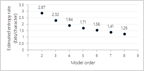
Estimated entropy rates using increasingly complex Markov models. As expected, the estimated entropy rate decreases as the order of the model (i.e. the number of characters being taken into account) increases.
Note that, because the Markov model being constructed is based on a necessarily finite corpus of textual samples, estimating the entropy rate for large values of \(n\) will yield artificially low information rates. Indeed, increasing the order of the model will decrease the number of samples per \(n\)-letters prefix, to the point that for very large values of \(n\), knowledge the first \(n-1\) letters of a passage uniquely identifies the passage in question, deterministically yielding the \(n\)th letter.
In the graph presented above, it is therefore likely that the estimates for \(n\) over 5 or 6 are already plagued by a significant amount of sampling error; indeed, for any given \(n\) there are in total \(27^{n}\) possible \(n\)-grams consisting only of the 26 alphabetic letters and a space, which exceeds the size of the corpus used in this experiment as soon as \(n > 5\).
Extrapolating these results to large values of \(n\) is particularly tricky, as in the general case nothing is known about the shape of this sequence of values except for the fact that it’s positive decreasing: deriving the limit entropy rate from this set of measurements requires building a model of the consecutive estimates, and fitting this model to the measured estimates.
As a rough example, call this sequence of values \(F_k\) and assume that it verifies the recurrence equation \(F_{k+1} – F_k = \alpha (F_{n} – F_{n-1})\). Then the \(\alpha\) that yields the best approximation (taking the two initial values for granted since they are less likely to suffer from sampling errors) is \(\alpha \approx 0.68\) (\(\mathcal{L}^2\) error: \(6.7 · 10^{-3}\)), and the corresponding entropy rate is \(h \approx 1.14\) bits/character.
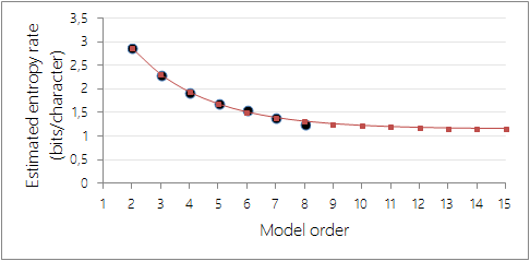
Extrapolated entropy rate values for \(\alpha \approx 0.68\). In this heuristic model, the limit entropy rate is \(h \approx 1.14\) bits/character.
Generating fake English text
The statistical model of English built in the previous section can be used to generate fake English text : to this end, we introduce a pick function that, given a Counter (that is, a mapping from elements to numbers of occurrences), picks an element at random, respecting the distribution described by that Counter object.
	import random
	def pick(counter):
		sample, accumulator = None, 0
		for key, count in counter.items():
			accumulator += count
			if random.randint(0, accumulator - 1) < count:
				sample = key
		return sample
A detailed explanation of this function will be the subject of a later post: efficiently sampling from an unordered, non-uniformly distributed sequence without pre-processing it is a non-trivial problem.
Given a length-\(n\) prefix, the generation algorithm obtains a new token by sampling from the distribution of tokens directly following this prefix. The token thus obtained is then appended to the prefix and the first token of the prefix is dropped, thus yielding a new prefix. The procedure is then repeated as many times as the number of characters that we want to obtain.
The following snippet implements this logic: model is a model obtained using the previously listed functions, state is the initial prefix to use, and length is the number of tokens that we want to generate.
	def generate(model, state, length):
		for token_id in range(0, length):
			yield state[0]
			state = state[1:] + (pick(model[state]), )
All that remains to be done is to pick a random initial prefix, using pick once again (the fill function wraps text at 80 columns to make the display prettier):
	prefix = pick(stats)
	gibberish = "".join(generate(model, prefix, 100)

	import textwrap
	print(textwrap.fill(gibberish))
Results: a collection of random Shakespeare samples
Feeding the whole of Shakespeare’s works into the model yields the following samples. Note how increasing the order of the model yields increasingly realistic results.
\(n=2\): second-order approximation
me frevall mon; gown good why min to but lone’s and the i wit, gresh, a wo. blace. belf, to thouch theen. anow mass comst shou in moster. she so, hemy gat it, hat our onsch the have puck.
\(n=3\): third-order approximation
glouces: let is thingland to come, lord him, for secress windeepskirrah, and if him why does, we think, this bottle be a croyal false we’ll his bein your be of thou in for sleepdamned who cond!
\(n=5\): fifth-order approximation
a gentlewomen, to violence, i know no matter extinct. before moment in pauncheon my mouth to put you in this image, my little join’d, as weak them still the gods! she hath been katharine; and sea and from argies, in the sun to be a strawberries ‘god servant here is ceremonious and heard.
\(n=8\): eigth-order approximation
gloucester, what he was like thee by my lord, we were cast away, away! mark that seeth not a jar o’ the tiger; take it on him as i have, and without control the whole inherit of this.
Words as tokens
The code above defines tokens as characters, and builds a model of sequences of \(n\) consecutive characters. Yet, to generate more realistic-looking text, we can also split the training corpus by words, using
	model, stats = markov_model(words('sample.txt', encoding='utf-8'), 3)
	print(textwrap.fill(" ".join(generate(model, pick(stats), 100))))
Here’s an example of a statistically sound sequence of English words, generated using a Markov model of order 3 of Shakespeare’s writings:
Third-order word approximation
he rouseth up himself and makes a pause while she the picture of an angry chafing boar under whose sharp fangs on his back doth lie an image like thyself all stain’d with gore whose blood upon the fresh flowers being shed doth make them droop with grief and extreme age.
Conclusion
Shannon’s 1948 article laid the foundations of a whole new science, information theory. The original paper is an easy yet extremely interesting read; it extends the notions presented here to derive theorems that link source entropy to the maximal possible compression of a source, and goes on to describe a mathematical framework for error correction.
Shannon himself also worked on the estimation of the information rate of English. However, since large-scale statistical experiments were impractical then, Shannon instead constructed an experiment involving humans: subjects were asked to guess the letters of a text one by one, and incorrect guesses per character were recorded to estimate the source entropy of sentences; in this experimental setting Shannon obtained a an estimate of the information rate of English between 0.6 and 1.3 bits per letter, in line with the results presented in this article.
Want to experiment by yourself? Download the full source code (also available for python 2.7)!
Did you find the initial quote hard to decipher? Does that pseudo-Shakespeare text look realistic? Do you know other beautiful applications of information theory? Let us know in the comments!
Thank you so much for posting this! A digital-humanities literary historian at Stanford has been posting some fascinating graphics of what he says are the second-order word redundancies of hundreds and thousands of major (and minor) British novels, calculated using bigram frequencies of their plain text files, but he doesn’t say how he is doing his math–and I have been stumped trying to replicate his calculations. Your code, which I have been playing with, seems to take me a long way forward. Now to figure out how to calculate redundancy given entropy!
If you are curious, the Stanford work is published at https://litlab.stanford.edu/LiteraryLabPamphlet11.pdf
The redundancy stuff starts on page 5
Hello
Thank you for giving a clear and concise explanation of information theory and especially the code. I am doing a final year project on information theory whilst trying to do the experiment for myself it somewhat harder to run as it is giving me an error
Thank you
Awesome post … thank you.
Wow, that’s a good article. What is the background of the problem?