After introducing true and pseudo-random number generators, and presenting the methods used to measure randomness, this article details a number of common statistical tests used to evaluate the quality of random number generators.
Introduction: true and pseudo-random number generators
Obtaining long sequences of random numbers, as required by some cryptographic algorithms, is a delicate problem. There are basically two types of random number generators: true random number generators, and pseudo-random number generators.
This article assumes no particular knowledge about the generation of random numbers, so if you already know about TRNGs and PRNGs, you may want to skip to the core of this article.
True random number generators (TRNGs)
True random number generators rely on a physical source of randomness, and measure a quantity that is either theoretically unpredictable (quantic), or practically unpredictable (chaotic — so hard to predict that it appears random).
I’ve compiled a list of sources of true randomness (capable of sufficiently fast output); please let me know in the comments if I forgot any.
- Thermal noise, due to the thermal agitation of charge carriers in an electronic component, and used by some Intel RNGs
- Imaging of random processes, used by LavaRnd
- Atmospheric noise, mostly due to thunder storms happening around the globe, and used by random.org
- Cosmic noise, due to distant stars and background radiation
- Driver noise, often used by
/dev/randomin Unix-like operating systems ((See this post by Arnold Reinhold for a discussion on how to manually increase the entropy of/dev/random)) - Transmission by a semi-transparent mirror, used by randomnumbers.info
- Nuclear decay, used by HotBits
- Coupled inverters, used by Intel’s new random generators.
The coupled inverters technique devised by Greg Taylor and George Cox at Intel is truly the most fascinating one : it relies on collapsing the wave function of two inverters put in a superposed state.
Pseudo-random number generators (PRNGs)
Pseudo-random number generators are very different: they act as a black box, which takes one number (called the seed ((The current system time is commonly used as a default seed, although for more security-sensitive applications user input is sometimes used (most often by asking the user to shake their mouse in a random fashion) )) and produces a sequence of bits; this sequence is said to be pseudo-random if it passes a number of statistical tests, and thus appears random. These tests are discussed in the following section; simple examples include measuring the frequency of bits and bit sequences, evaluating entropy by trying to compress the sequence, or generating random matrices and computing their rank.
Formal definition
A pseudo random number generator is formally defined by an initialization function, a state (a sequence of bits of bounded length), a transition function, and an output function:
- The initalisation function takes a number (the seed), and puts the generator in its initial state.
- The transition function transforms the state of the generator.
- The output function transforms the current state to produce a fixed number of bit (a zero or a one).
A sequence of pseudo-random bits, called a run, is obtained by seeding the generator (that is, initializing it using a given seed to put it in its initial state), and repeatedly calling the transition function and the output function. ((By definition, since the number of possible states is bounded, this sequence will be periodic; in practice however, this period can be made as large as desired by increasing the number of bits in the state.)) This procedure is illustrated by the following diagram:
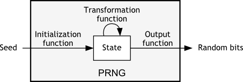
Schematic diagram of a pseudo-random number generator
In particular, this means that the sequence of bits produced by a PRNG is fully determined by the seed ((This property is very useful when using PRNGs to simulate experiments; seeds used during the simulation are recorded in case the results of one specific run need to be reproduced)). This has a few disagreeable consequences, among which the fact that a PRNG can only generate as many sequences as it can accept different seeds. Thus, since the range of values that the state can take is usually much wider than that of the seed, it is generally best to only seldom reset (re-seed) the generator ((except when the state risks being compromised — see the following section)).
Cryptographically secure pseudo-random number generators
Since PRNGs are commonly used for cryptographic purposes, it is sometimes asked that the transformation and output functions satisfy two additional properties :
- Un-predictability: given a sequence of output bits, the preceding and following bits shouldn’t be predictable
- Non-reversibility: given the current state of the PRNG, the previous states shouldn’t be computable.
Rule 1 ensures that eavesdropping the output of a PRNG doesn’t allow an attacker to learn more than the bits they overheard.
Rule 2 ensures that past communications wouldn’t be compromised should an attacker manage to gain knowledge of the current state of the PRNG (thereby compromising all future communications based on the same run).
When a PRNG satisfies these two properties ((Again, saying that a PRNG satisfies these properties means that either it can be proven that the rules cannot be broken, or that it is not practically possible to break them in a reasonable amount of time)), it is said to be cryptographically secure ((cryptographically secure pseudo-random number generators are often abbreviated as CSPRNGs)).
Testing pseudo-random number generators
There are a number of statistical tests devised to distinguish pseudo-random number generators from true ones; the more a PRNG passes, the closer it is considered to be from a true random source. This section presents general methodology, and studies a few example tests.
Testing methodology
Testing a single sequence
Almost all tests are built on the same structure: the pseudo-random stream of bits produced by a PRNG is transformed (bits are grouped or rearranged, arranged in matrices, some bits are removed, …), statistical measurements are made (number of zeros, of ones, matrix rank, …), and these measurements are compared to the values mathematically expected from a truly random sequence.
More precisely, assume that \(f\) is a function taking any finite sequence of zeros and ones, and returning a non-negative real value. Then, given a sequence of independent and uniformly distributed random variables \(X_n\), applying \(f\) to the finite sequence of random variables \((X_1, …, X_n)\) yields a new random variable, \(Y_n\). This new variable has a certain cumulative probability distribution \(F_n(x) = \mathbb{P}(Y_n \leq x)\), which in some cases approaches a function \(F\) as \(n\) grows large. This limit function \(F\) can be seen as the cumulative probability distribution of a new random variable, \(Y\), and in these cases \(Y_n\) is said to converge in distribution to \(Y\).
Randomness tests are generally based on carefully selecting such a function ((In particular, the function is often chosen so that the limit random variable \(Y\) has a monotonous (decreasing) density function)), and calculating the resulting limit probability distribution. Then, given a random sequence \(\epsilon_1, \ldots, \epsilon_n\), it is possible to calculate the value of \(y = f(\epsilon_1, \ldots, \epsilon_n)\), and assess how likely this value was by evaluating the probability \(\mathbb{P}(Y \geq y)\) — that is, the probability that a single draw of the limit random variable \(Y\) yields a result greater than or equal to \(y\). If this probability is lower than \(0.01\), the sequence \(\epsilon_1, \ldots, \epsilon_n\) is said to be non-random with confidence 99%. Otherwise, the sequence is considered random.
An example: the bit frequency test
Let \((X_n)\) be an infinite sequence of independent, identically distributed random variables. Take \(f\) to be \(f(x_1, …, x_n) = \frac{1}{\sqrt{n}} \sum_{k=1}^n \frac{x_n – \mu}{\sigma}\) where \(\mu\) is the average, and \(\sigma\) the standard deviation, of any \(X_k\). Define \(Y_n = f(X_1, …, X_n)\). The central limit theorem states that the distribution of \(Y_n\) tends to the standard normal distribution. This theorem is illustrated below.
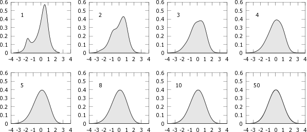
Example of convergence in distribution to the standard normal distribution, after summing 1, 2, 3, 4, 5, 8, 10, and 50 independent random variables following the same distribution.
Consider the particular case where \(X_n\) is uniformly distributed over the discrete set \(\{-1,1\}\). The central limit theorem applies, and \(Y_n = f(X_1, …, X_n)\) converges in distribution to the standard normal law. For practical reasons, however, we choose to consider \(Y_n = |f(X_1, …, X_n)|\), which converges in distribution to a variable \(Y_\infty\). \(Y_\infty\) has the half-normal distribution (illustrated on the left), which has the nice property of being monotonically decreasing.
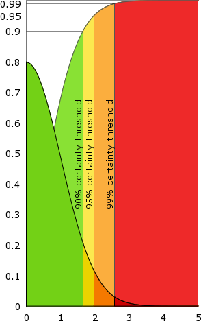
In plain colours, the half-normal distribution. In pale colours, the corresponding cumulative distribution function. If a pseudo-random sequence is picked in the red area, it is declared non-random with 99% certainty (the yellow and orange areas correspond to a certainty of 90% and 95% respectively).
Here is how the test proceeds : the sequence \((\epsilon_1, \ldots, \epsilon_n)\) given by the PRNG is converted to a sequence of elements of \(\{-1, 1\}\) by changing each \(\epsilon_i\) to \(x_i = 2 \cdot \epsilon_i – 1\). This gives \(x_1, \ldots, x_n\). Then, \(|f(x_1, \ldots, x_n)| = \left|\sum_{k=1}^n \frac{x_k}{\sqrt{n}}\right|\) is numerically calculated, yielding \(y\). Finally, the theoretical likeliness of a truly random sequence yielding a value equal to or greater than \(y\) is evaluated using the cumulative distribution function of \(Y_\infty\) (in pale colours).
If this probability is too low (red area, probability below \(0.01\)), the sequence is rejected as non-random, with 99% certainty. If it is greater than \(0.01\), but less than \(0.05\) (orange area) the sequence is sometimes ((Some papers advise to reject any sequence with a p-value \(\leq 0.05\), but most choose \(0.01\) as the threshold)) rejected as non-random with 95% certainty. Similarly, if it is greater than \(0.05\) but less than \(0.10\) (yellow area), the sequence is sometimes rejected as non-random, with 90% certainty.
High probabilities (green area, probabilities greater than \(0.10\)), finally, do not permit to distinguish the pseudo-random sequence from a truly random one ((Note that this generates false positives: a true random number generator will, in the long run, produce every possible sequence: sequences yielding measurements that fall in the red area will be rare, but they will occur, and will be discarded as non-random. This is very important to the PRNG-testing procedure, as explained in the next sub-section)).
Testing a pseudo-random number generator
To test whether a pseudo-random number generator is close to a true one, a sequence length is chosen, and \(m\) pseudo-random sequences of that length are retreived from the PRNG, then analysed according to the previous methodology. It is expected, if the confidence level is 1%, that about 99% of the sequences pass, and 1% of the sequences fail; if the observed ratio significantly differs from 99 to 1, the PRNG is said to be non-random. More precisely, the confidence interval is generally chosen to be \(p \pm 3\frac{\sqrt{p(1-p)}}{\sqrt{m}}\), where \(p\) is the theoretical ratio (99% here); this takes the probability of incorrectly rejecting a good number generator down to 0.3%.
This confidence interval is obtained as follows. For large values of \(m\), approximate the probability of rejecting \(r\) sequences by \(\binom{m}{r} p^{1-r} (1-p)^r\) (here \(p = 99\%\)). Write \(\sigma_i\) the random variable denoting whether the \(i\)th sequence was rejected. Then with the previous approximation all \(\sigma_i\) are independent and take value \(0\) with probability \(p\), \(1\) with probability \(1-p\) (standard deviation: \(\sqrt{p(1-p)}\)). The central limit theorem states that with probability close to \(\displaystyle \int_a^b \frac{e^{-x^2/2}}{\sqrt{2\pi}}\), the observed rejection frequency \(\hat{p}\) lies in the interval \(\left[p + b\frac{\sqrt{p(1-p)}}{\sqrt{m}}, p + a\frac{\sqrt{p(1-p)}}{\sqrt{m}}\right]\). Finally, setting \(b = -a\) and adjusting \(a\) so that this probability is \(\approx 99.7\%\) yields \(a \approx 3\).
Tests suites
A number of test suites have been proposed as standards. The state-of-the-art test suite was for a long time the DieHard test suite (designed by George Marsaglia), though it as eventually superseeded by the National Institute of Standards and Technology recommendations. Pierre l’Ecuyer and Richard Simard, from Montreal university, have recently published a new collection of tests, TestU01, gathering and implementing a impressive number of previously published tests and adding new ones. ((Ent is another implementation of a few tests.))
A subset of these tests is presented below.
A list of common statistical tests used to evaluate randomness
Equidistribution (Monobit frequency test, discussed above)
Purpose: Evaluate whether the sequence has a systematic bias towards 0 or 1 (real-time example on random.org)
Description: Verify that the arithmetic mean of the sequence approaches \(0.5\) (based on the law of large numbers). Alternatively, verify that normalized partial sums \(s_n = \frac{1}{\sqrt{n}} \sum_{k=1}^n \frac{2\cdot\epsilon_k – 1}{\sqrt{2}}\) approach a standard normal distribution (based on the central limit theorem).
Variants: Block frequency test (group bits in blocks of constant length and perfom the same test), Frequency test in a block (group bits in blocks of constant length and perform the test on every block).
Runs test
Purpose: Evaluate whether runs of ones or zeros are too long (or too short) (real-time example on random.org)
Description: Count the number of same-digits blocks in the sequence. This should follow a binomial distribution \(\mathcal{B}(n, 1/2)\). By noting that the number of same-digits blocks is the sum of the \(\sigma_i\) where \(\sigma_i = 1\) if \(\epsilon_i \not= \epsilon_{i+1}\) and \(\sigma_i = 0\) otherwise, the previous method can be applied.
Variants: Longest run of ones (divide the sequence in blocks and measure the longest run of ones in each block).
Binary matrix rank
Purpose: Search for linear dependencies between successive blocks of the sequence
Description: Partition the sequence in blocks of length \(n \times p\). Build one \(n \times p\) binary matrix from each block, and compute its rank. The theoretical distribution of all ranks is however not easy to compute — this problem is discussed in details in a paper by Ian F. Blake and Chris Studholme from the university of Toronto.
Discrete Fourier transform
Purpose: Search for periodic components in the pseudo-random sequence
Description: Compute a discrete Fourier transform of the pseudo-random input \(2\epsilon_1 – 1, \ldots, 2\epsilon_n – 1\), and take the modulus of each complex coefficient ((Note that, since the input sequence is real-valued, its DFT is symetrical; hence all the counting need only happen on the first half of the DFT sequence)). Compute the 95% peak height threshold value, defined to be the theoretical value that no more than 5% of the previously calculated moduli should exceed (\(\sqrt{-n\log(0.05)}\) (NIST)), and count the actual number of moduli exceeding this threshold. Assess the likeliness of such a value.
Compressibility (Maurer’s universal statistical test)
Purpose: Determine whether the sequence can be compressed without loss of information (evaluate information density). A random sequence should have a high information density.
Description: Partition the sequence in blocks of length \(L\), and separate these block into categories. Call the first \(Q\) blocks the initialisation sequence, and the remaining \(K\) blocks the test sequence. Then, give each block in the test sequence a score equal to the distance that separates it from the previous occurence of a block with the same contents, and sum the binary logarithm of all scores. Divide by the number of blocks to obtain the value of the test function, and verify that this value is close enough to the theoretically expected value. ((Since the binary logarithm is concave, this value gets smaller as the dispersion of the scores increase; informally, since the expected distance between to blocks of equal contents is approximately the number of possible different blocks (\(2^L\) ) the expected value should be about \(\log_2(2^L)\) — that is \(L\). Computing the actual expected values yields a somewhat smaller number, which approaches \(L – 0.83\) as \(L \to \infty\) (Coron, Naccache) ))
Maximum distance to zero, Average flight time, Random excursions
Purpose: Verify that the sequence has some of the properties of a truly random walk
Description: Consider the pseudo-random sequence to represent a random walk starting from zero and moving up (down) by one unit every time a zero (a one) occurs in the sequence. Measure the maximum height reached by the walk, as well as the average time and the number of states visited. Also, for each possible state (integer), measure in how many cycle it appears. Evaluate the theoretical probability of obtaining these values.
The sources previously cited (in particular the NIST recommendation paper) present mathematical background about these tests, as well as lots of other tests.
Did I miss your favourite randomness test? Were you ever confronted to obvious imperfections in a pseudo-random number generator? Tell us in the comments!
Dear Sir, I have some PRNG datasets available, would you please consider evaluating the datasets that I put available?
Pingback: Monte Carlo: what is a seed? - PhotoLens