 Children’s cereal manufacturers often attract the attention of young clients by including small prizes and toys in every box; sometimes all prizes are identical, but most often individual prizes are part of a collection, and kids are encouraged to collect them and try to complete a full collection. How long does it take ?
Simple probabilistic modeling shows that on average \(n (1 + 1/2 + \ldots + 1/n)\) boxes are required to complete a full set of \(n\) prizes: for example, it takes on average \(14.7\) boxes to complete a full set of six prizes.
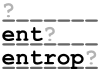 Thanks to the verbosity of the English language, proficient English speakers generally find it relatively easy to decipher the above passage despite the numerous omissions.
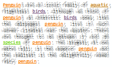 Most linear-time string searching algorithms are tricky to implement, and require heavy preprocessing of the pattern before running the search. This article presents the Rabin-Karp algorithm, a simple probabilistic string searching algorithm based on hashing and polynomial equality testing, along with a Python implementation. A streaming variant of the algorithm and a generalization to searching for multiple patterns in one pass over the input are also described, and performance aspects are discussed.
 TL;DR: I’ve taken plenty of notes while developing my
 .png) Comparing strings is often — erroneously — said to be a costly process. In this article I derive the theoretical asymptotic cost of comparing random strings of arbitrary length, and measure it in C, C++, C# and Python.
Comparing strings is often — erroneously — said to be a costly process. In this article I derive the theoretical asymptotic cost of comparing random strings of arbitrary length, and measure it in C, C++, C# and Python.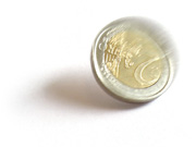 In a famous article published 1951 ((Various techniques used in connection with random digits. NIST journal, Applied Math Series, 12:36-38, 1951. This article does not seem to be available online, though it is widely cited. It is reprinted in pages 768-770 of Von Neumann’s collected works, Vol. 5, Pergamon Press 1961)), John Von Neumann presented a way of skew-correcting a stream of random digits so as to ensure that 0s and 1s appeared with equal probability. This article introduces a simple and mentally workable generalization of his technique to random dice, so a loaded die can be used to uniformly draw numbers from the set \(\{1, 2, 3, 4, 5, 6\}\), with reasonable success.
 Most cafeteria water dispensers will let two (sometimes more) people fill a jug at the same time. This article uses simple maths to prove that it’s a waste of time. In other words, two people should never use the same water dispenser at the same time: I call this the cafeteria paradox.
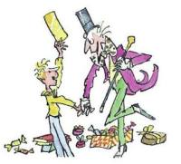 There’s something that has troubled me since childhood. In Charlie and the chocolate factory, one of the lucky children (Veruca Salt) gets her golden ticket thanks to her father repruposing his peanut shelling factory in a chocolate-bar-unwrapping factory.