Children’s cereal manufacturers often attract the attention of young clients by including small prizes and toys in every box; sometimes all prizes are identical, but most often individual prizes are part of a collection, and kids are encouraged to collect them and try to complete a full collection. How long does it take ?

Simple probabilistic modeling shows that on average \(n (1 + 1/2 + \ldots + 1/n)\) boxes are required to complete a full set of \(n\) prizes: for example, it takes on average \(14.7\) boxes to complete a full set of six prizes.

Numerical and experimental simulation

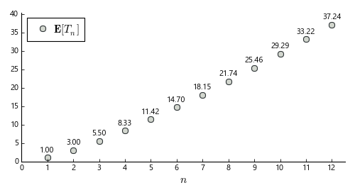
The expected number of boxes to buy before finding all \(n\) prices is shown below:

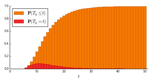
And here is an experimental simulation for \(n = 6\): the graph below shows how many purchases were required to obtain six prizes out of six, over 1,000,000 simulations.

Interested in how these plots were obtained? Read on to find out, or skip directly to the comments to share your thoughts!

Calculations and simulation code

Theoretical average

Assume there are \(n\) different prizes, all of which are equally distributed in cereal boxes. Model buyer behavior as a sequence of purchases, and call \(T_k\) the time at which they find the \(k\)^th prize : clearly \(T_0 = 0\) (no purchases are needed to find 0 prizes) and \(T_1 = 1\) (one finds their first prize immediately after buying their first cereal box). Naturally, \(T_n\) denotes the time required to find all prizes.

To calculate \(\newcommand{\E}[1]{\mathrm{\mathbf{E}}\left[#1\right]}\E{T_n}\), call \(\Delta_k\) the elapsed time between the \(k\)^th and \(k+1\)^th prizes, i.e. \(\Delta_k = T_{k+1} – T_k\). Summing over \(k\) yields \(\sum_{k=0}^{n-1} \Delta_k = T_n – T_0\) which, given the linearity of the expectation operator, yields $$
\sum_{k=0}^{n-1} \E{\Delta_k} = \E{T_n}
$$

All that remains to be done now is to calculate \(\E{\Delta_k}\) for all \(k \in \{ 0, \ldots, n-1 \}\). By definition $$
\newcommand{\P}[1]{\mathrm{\mathbf{P}}\left(#1\right)}\E{\Delta_k} = \sum_{\delta = 1}^\infty \P{T_{k+1} = T_{k} + \delta} · \delta
$$

\(\P{T_{k+1} = T_{k} + \delta}\) is the probability of finding the \(k+1\)^th exactly \(\delta\) purchases after obtaining the \(k\)^th; that is, the probability of completing \(\delta – 1\) unproductive purchases, then a successful one. Now the probability of hitting a sequence of \(\delta – 1\) unproductive purchases is exactly \((k/n)^{\delta-1}\); hence $$
\P{T_{k+1} = T_{k} + \delta} = \left(\frac{k}{n}\right)^{\delta-1}\left(1 – \frac{k}{n}\right)
$$

Summing over positive values of \(\delta\) yields $$
\begin{align*}
\E{\Delta_k} &= \sum_{\delta = 1}^\infty \P{T_k = T_{k-1} + \delta} · \delta = \sum_{\delta = 1}^\infty (k/n)^{\delta-1} · (1 – k/n) · \delta\\
&= (1 – k/n) \sum_{\delta = 1}^\infty \delta (k/n)^{\delta-1} = (1 – k/n) \frac{1}{(1 – k/n)^2}\\
&= \frac{1}{1 – k/n} = \frac{n}{n-k}
\end{align*}
$$

And summing over \(k\) yields $$
\begin{align*}
\E{T_n} &= \sum_{k=0}^{n-1} \E{\Delta_k} = \sum_{k=0}^{n-1} \frac{n}{n-k} = n \sum_{k=1}^{n} \frac{1}{k}\\
&= n \left(1 + \frac12 + \frac13 + \ldots + \frac1{n}\right)
\end{align*}
$$

Which, for large \(n\), is \(n \left(\log(n) + \gamma + \frac1{2n} + o\left(\frac1n\right)\right)\) (where \(\gamma \approx 0.57722\) denotes the Euler–Mascheroni constant).

Note that, as expected, \(\E{\Delta_k}\) quickly increases as \(k\) grows larger: the more prizes have already been found, the harder it is to get a new one, to the point that finding the last prize requires \(n\) purchases on average.

Numerical simulations

The experimental data above was simulated using the following code:

	repeat = 1000*1000
	time_to = defaultdict(Counter)
	
	for _ in range(repeat):
		purchased = 0
		collected_prizes = set()
		
		while len(collected_prizes) < n: # Until all prizes have been found
			purchased += 1 # Purchase one more box
			prize = random.randint(1, n) # Open it
			if prize not in collected_prizes: # Is it a new prize ?
				time_to[len(collected_prizes) + 1][purchased]  += 1 # Yes, count it !
				collected_prizes.add(prize)	# And add it to list of already found prizes

Conclusion

One might want to find some intuitive way to comprehend the formula derived above, \(\E{T_n} = n\left(1 + 1/2 + \ldots + 1/n\right)\). A relatively easy way to get such an intuition is to summarize the calculation above, realizing that each new packet bought after finding the \(k\)^th prize brings an extra prize with probability \((n-k)/n\) ; since each purchase is independent, it takes on average \(n / (n-k)\) purchases to find a new prize; then summing over \(k\) yields the final formula.

Have you ever completed a full set of cereal box prizes? How long did it take?